Getting Started with Variable
Imports
from leavitt.timeseries import Variable
from leavitt.utils import phase_fold, plot_phased_lightcurve
There are two main ways to initialize a Variable object.
Using the NSC ID (objectid) of a star. We’ll do that here. This performs a synchronous query to the DataLab catalog.
Giving it a TimeSeries object.
star = Variable('150537_4644')
This object now has an attribute called timeseries which contains the timeseries data.
star.timeseries
time |
mag_auto |
magerr_auto |
filter |
exptime |
|---|---|---|---|---|
Time |
float64 |
float64 |
str1 |
int64 |
57113.05614621984 |
15.811543 |
0.001926 |
i |
150 |
57112.05490842834 |
15.801223 |
0.001874 |
r |
150 |
57112.13323347038 |
15.954048 |
0.002102 |
g |
150 |
57113.08296847297 |
15.759274 |
0.001752 |
g |
150 |
57112.25814789068 |
16.2586 |
0.002162 |
g |
150 |
… |
… |
… |
… |
… |
57112.27053951612 |
16.24863 |
0.002241 |
g |
150 |
57113.00249109836 |
15.955009 |
0.001944 |
g |
150 |
57112.22724048141 |
16.239832 |
0.002429 |
g |
150 |
57112.20861871168 |
16.207851 |
0.002292 |
g |
150 |
57112.22103560204 |
16.228163 |
0.002224 |
g |
150 |
Periodogram
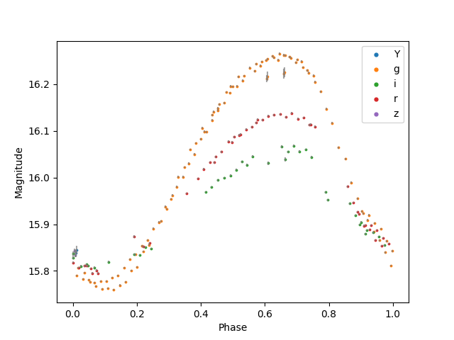
Now, we can perform a Lomb-Scargle multiband to find the period of the star (it may take a while). This is a RRc star with a period of 0.3367 days.
frequency, power = star.ls_mb_periodogram()
period, error = star.get_period(frequency, power)
The period and errors are stored in the new variables, but also a new attribute called period that stores the period only.
print('{:.5f} +/- {:.5f} days'.format(period.value,error.value))
print('{:.5f} days'.format(star.period.value))
0.33667 +/- 0.00004 days
0.33667 days
We can now get the data to construct a phased lightcurve.
phase = phase_fold(star.timeseries['time'],period)
plot_phased_lightcurve(phase, star.timeseries['mag_auto'],mags_errs=star.timeseries['magerr_auto'],filters=star.timeseries['filter'])